How to calculate the effective mass according to the wien mailinglist

[Wien] Effective mass calculation

Marcelo Barbosa Thu, 16 Nov 2017 00:59:11 -0800

Dear Sirs,

I’m having some trouble calculating the effective mass using the results from 
the band structure, so I’m going to explain the procedure that I tried.

First I compared the band structure with previous simulations and experimental 
results and it is correct.
Looking into the file case.spaghetti_ene, I can confirm that the k-points are 
in units of 2*pi/bohr (as explained in 
https://www.mail-archive.com/wien@zeus.theochem.tuwien.ac.at/msg05273.html 
<https://www.mail-archive.com/wien@zeus.theochem.tuwien.ac.at/msg05273.html>).
Therefore, in order to fit the curve to the parabolic function E = hbar^2 * k^2 
/ (2 * m) to get the value of m, I transformed the 4th column from Bohr to 
Angstrom by multiplying it by 1.8897259886, squared it and subtracted to the 
5th column the energy value at k=0 to have E(k=0) = 0.
If I plot the resulting E vs k^2, I get a straight line for the first few 
points and so I calculate the slope in that range, which is around 9.9.
Then, using the relation m = hbar^2 / (2 * slope), using hbar in units of eV.s 
I calculate the effective mass.
The result I get is 0.024*me when I was expecting to get something around 
0.28*me, so I’m wrong in one order of magnitude.
Could you please help me understand what I’m doing wrong?

Best regards,
Marcelo

Answer of Gavin Abo

Re: [Wien] Effective mass calculation

Gavin Abo Fri, 17 Nov 2017 01:45:58 -0800

Instead of plotting E [eV] vs k^2 [(2*pi/angstrom)^2], have you tried plotting E [J] vs k [pi/m]?

Take for example the plot at:

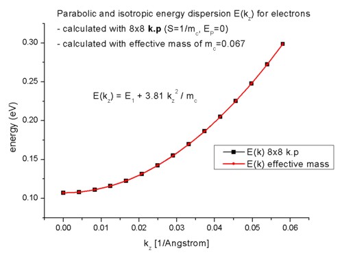
http://www.nextnano.com/nextnano3/images/tutorial/2Deffective_mass_vs_8x8kp/kz_dispersion_small.jpg

[ from http://www.nextnano.com/nextnano3/tutorial/2Dtutorial4.htm ]

Assume E has units of eV and k has units of pi/angstrom, such that:

k [pi/angstrom]     E [eV]
0    0.10707
0.005    0.108491642
0.01    0.112756567
0.015    0.119864776
0.02    0.129816269
0.025    0.142611045
0.03    0.158249104
0.035    0.176730448
0.04    0.198055075
0.045    0.222222985
0.05    0.249234179
0.055    0.279088657
0.06    0.311786418
0.065    0.347327463
0.07    0.385711791

Use 1 angstrom = 10^-10 m [ https://en.wikipedia.org/wiki/%C3%85ngstr%C3%B6m ] to convert k from angstroms to meters and 1 eV = 1.602*10^-19 J to convert E from eV to Joules [ https://en.wikipedia.org/wiki/Electronvolt ], such that:

k [pi/m]    E [J]
0.00E+00    1.71526E-20
5.00E+07    1.73804E-20
1.00E+08    1.80636E-20
1.50E+08    1.92023E-20
2.00E+08    2.07966E-20
2.50E+08    2.28463E-20
3.00E+08    2.53515E-20
3.50E+08    2.83122E-20
4.00E+08    3.17284E-20
4.50E+08    3.56001E-20
5.00E+08    3.99273E-20
5.50E+08    4.471E-20
6.00E+08    4.99482E-20
6.50E+08    5.56419E-20
7.00E+08    6.1791E-20

For example in Excel, plot the E [J] vs k [pi/m] values, add a Polynomial Trendline, and Display the Equation on chart [http://www.statisticshowto.com/excel-multiple-regression/ ].

This should give you a polynomial fit equation:

y = 9E-38*x^2 + 2E-20

The above is a second order polynomial equation of the form [https://en.wikipedia.org/wiki/Quadratic_function ]:

y = A*x^2 + B*x + C

where A = 9E-38, B = 0, and C = 2E-20.

Note that the y is the fitted energy on the y-axis and x is the k of x-axis:

E = 9E-38*k^2 + 2E-20

Use calculus to get the second derivative of E:

d^2 E / dk^2 = 2*A = 9E-38

hbar = 1.05*10^-34 J*s [ https://en.wikipedia.org/wiki/Planck_constant ]

me = 9.11*10^-31 [ https://en.wikipedia.org/wiki/Electron_rest_mass ]

Using the effective mass relation [ https://arxiv.org/abs/1605.01428v2 (equation 4)]:

m*=hbar^2/(2*A)

m*=[(1.05*10^-34)^2/(2*9E-38)]/(9.11*10^-31) = 0.067*me